Analysis of inflection points
Determines the relationship between treatment time
 and the two inflection point times,
 and
and  .
.
import sys,os
import numpy as np
import pandas as pd
import scipy.optimize as optim
import functions
import glob
from scipy.stats import gamma
import math
import matplotlib.pyplot as plt
from matplotlib import rcParams
import scipy.stats as st
import matplotlib.font_manager as font_manager
from scipy.stats import t

from matplotlib.lines import Line2D
def linear(x,a,b):
    return (a + b*x)
data_directory = './data/'
os.chdir(data_directory)
cwd = os.getcwd()

studies = glob.glob('Study*')

n = [int(s.lstrip('Study')) for s in studies]
n.sort()

studies = ['Study'+str(ni) for ni in n]
Specify inflection points to neglect from specific studies.
studies_to_neglect = {}

studies_to_neglect = {'Study1':[60],'Study2':[60],'Study3':[60],'Study4':[30],
                     'Study5':[30],'Study6':[60],'Study7':[60],'Study8':[],
                     'Study9':[],'Study10':[],'Study11':[],'Study12':[60]}
inflection_points = {}
dof = -2 # Two parameters in the linear models

for s in studies:
    os.chdir(s)

    inflection_points[s] = pd.read_csv('gompertz_inflection_points_summary.csv')

    for tH in studies_to_neglect[s]:
        tH_vals = inflection_points[s].index[inflection_points[s]['CT'] == tH].tolist()[0]

        inflection_points[s] = inflection_points[s].drop(inflection_points[s].index[tH_vals])

    dof += len(inflection_points[s]['CT'])

    os.chdir(cwd)
tinv = lambda p, df: abs(t.ppf(p/2,df))
ts = tinv(0.05,dof)
Relationship between and
.
th, t1s = [], []

for s in studies:
    th += inflection_points[s]['CT'].to_list()
    t1s += inflection_points[s]['T1'].to_list()

results = optim.curve_fit(linear,th,t1s,full_output=True)

popt, pcov = results[0], results[1]

x = np.linspace(0,80,100)
t1 = linear(x,popt[0],popt[1])

residual = linear(np.array(th),popt[0],popt[1]) - np.array(t1s)

norm_RSS = math.sqrt(np.dot(residual,residual)/(len(t1s)-2))

RSS_text = r's.d. = ' + str(round(norm_RSS,2)) + ' h'

res = st.linregress(th,t1s)
fitname = r'T1 = ' + str(round(res.slope,2)) + '$\mathrm{T_H}$ + ' + str(round(res.intercept,2))

x = np.linspace(0,80,100)
y = res.slope*x + res.intercept

r_text = r'$\mathrm{R}^2 = ' + str(round(res.rvalue**2,3)) + '$'
n_samples = 10000

s_is, i_is = [], []

t1_up = np.zeros(shape=x.shape)
t1_low = np.zeros(shape=x.shape)

rt1_up = np.zeros(shape=x.shape)
rt1_low = np.zeros(shape=x.shape)

effective_sigma = np.zeros(shape=x.shape)

for i in range(0,x.shape[0]):
    samples = []

    a_samples, b_samples = np.random.multivariate_normal(popt,pcov,n_samples).T

    for a_sample,b_sample in zip(a_samples,b_samples):
        samples.append(linear(x[i],a_sample,b_sample))

    sigma = np.std(samples)

    effective_sigma[i] = math.sqrt(sigma**2 + norm_RSS**2)

    ci95 = effective_sigma[i]*ts

    t1_low[i], t1_up[i] = t1[i] - ci95, t1[i] + ci95

    rt1_low[i], rt1_up[i] = t1[i] - sigma*ts, t1[i] + sigma*ts
all_markers = ["o","v","^","<",">","s","p","P","*","X","d","D"]

fig, axs = plt.subplots(figsize=(11,10))

rcParams['font.family'] = 'sans-serif'
rcParams['font.sans-serif'] = ['Times New Roman']

#marker_list = {'Study1':'o','Study2':'D','Study3':'s','Study4':'X','Study5':'P'}

for s,mark in zip(studies,all_markers):
    if '11' not in s:
        labelname = s.replace('Study','Study ')
        plt.plot(inflection_points[s]['CT'],inflection_points[s]['T1'],marker=mark,ms=10,color='black',alpha=0.5,linewidth=0,label=labelname)

plt.plot(x,y,linewidth=4,color='#880000',alpha=0.5)

plt.text(60,75,r_text,fontsize=24)
plt.text(60,50,RSS_text,fontsize=24)

plt.fill_between(x,t1_up,t1_low,alpha=0.15,color='#660000',linewidth=0.0)
plt.fill_between(x,rt1_up,rt1_low,alpha=0.2,color='#000088',linewidth=0.0)

plt.text(54,25,fitname,fontsize=22)
plt.plot(np.linspace(48,52,2),28*np.ones(2,),color='#660000',alpha=0.6,lw=3)

plt.xticks(size=26)
plt.yticks(size=26)
plt.xlabel(r'Treatment time, $\mathrm{T_H}$ (h)',size=26,labelpad=10)
plt.ylabel(r'1$^{\mathrm{st}}$ inflection point, T1 (h)',size=26,rotation=90,labelpad=10)
plt.xlim(-2,80)
plt.ylim(0,300)
plt.legend(frameon=False,prop={'size': 17,'family':'Times New Roman'},markerscale=1.25,handlelength=1.0,loc='upper left')
plt.tight_layout()

#plt.savefig('THT1.png',dpi=300)

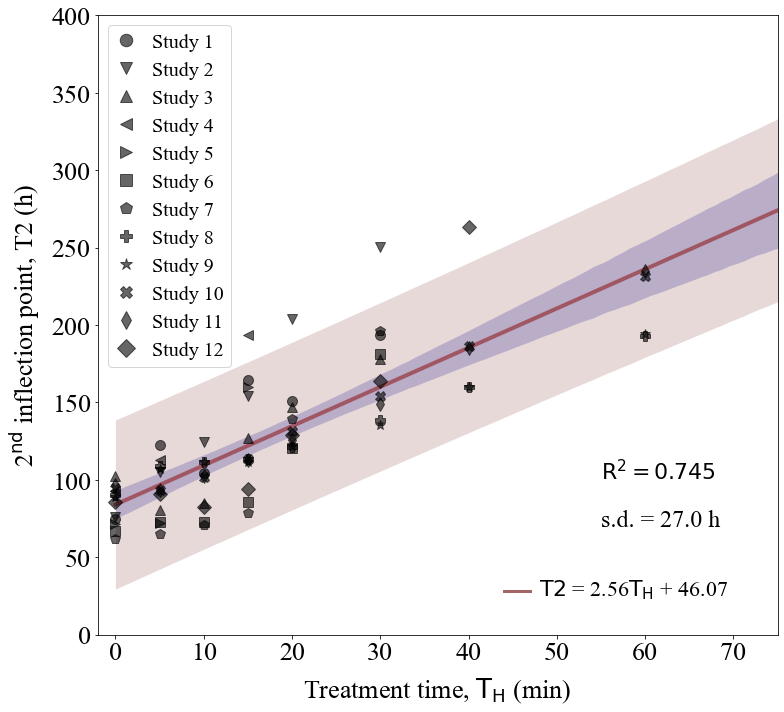
Relationship between and
.
th, t2s = [], []

for s in studies:
    th += inflection_points[s]['CT'].to_list()
    t2s += inflection_points[s]['T2'].to_list()

results = optim.curve_fit(linear,th,t2s,full_output=True)

popt, pcov = results[0], results[1]

x = np.linspace(0,80,100)
t2 = linear(x,popt[0],popt[1])

residual = linear(np.array(th),popt[0],popt[1]) - np.array(t2s)

norm_RSS = math.sqrt(np.dot(residual,residual)/(len(t2s)-2))

RSS_text = r's.d. = ' + str(round(norm_RSS,2)) + ' h'
fitname = r'$\mathrm{T2}$ = ' + str(round(res.slope,2)) + '$\mathrm{T_H}$ + ' + str(round(res.intercept,2))

r_text = r'$\mathrm{R}^2 = ' + str(round(res.rvalue**2,3)) + '$'
n_samples = 10000

s_is, i_is = [], []

t2_up = np.zeros(shape=x.shape)
t2_low = np.zeros(shape=x.shape)

rt2_up = np.zeros(shape=x.shape)
rt2_low = np.zeros(shape=x.shape)

effective_sigma = np.zeros(shape=x.shape)

for i in range(0,x.shape[0]):
    samples = []

    a_samples, b_samples = np.random.multivariate_normal(popt,pcov,n_samples).T

    for a_sample,b_sample in zip(a_samples,b_samples):
        samples.append(linear(x[i],a_sample,b_sample))

    sigma = np.std(samples)

    effective_sigma[i] = math.sqrt(sigma**2 + norm_RSS**2)

    ci95 = effective_sigma[i]*ts

    t2_low[i], t2_up[i] = t2[i] - ci95, t2[i] + ci95

    rt2_low[i], rt2_up[i] = t2[i] - sigma*ts, t2[i] + sigma*ts
fig, axs = plt.subplots(figsize=(11,10))

rcParams['font.family'] = 'sans-serif'
rcParams['font.sans-serif'] = ['Times New Roman']

plt.plot(x,t2,linewidth=4,color='#880000',alpha=0.5)#,label=fitname)

for s,mark in zip(studies,all_markers):
    labelname = s.replace('Study','Study ')
    plt.plot(inflection_points[s]['CT'],inflection_points[s]['T2'],marker=mark,ms=10,color='black',alpha=0.6,linewidth=0,label=labelname)

plt.text(55,100,r_text,fontsize=22)
plt.text(55,70,RSS_text,fontsize=24)

plt.text(48,25,fitname,fontsize=22)

plt.plot(np.linspace(44,47,2),28*np.ones(2,),color='#660000',alpha=0.6,lw=3)

plt.fill_between(x,t2_up,t2_low,alpha=0.15,color='#660000',linewidth=0.0)
plt.fill_between(x,rt2_up,rt2_low,alpha=0.2,color='#000088',linewidth=0.0)

plt.xticks(size=26)
plt.yticks(size=26)
plt.xlabel(r'Treatment time, $\mathrm{T_H}$ (min)',size=26,labelpad=10)
plt.ylabel(r'2$^{\mathrm{nd}}$ inflection point, T2 (h)',size=26,rotation=90,labelpad=10)
plt.xlim(-2,75)
plt.ylim(0,400)
plt.legend(frameon=True,prop={'size': 20,'family':'Times New Roman'},markerscale=1.25,handlelength=1.0,loc='upper left')
plt.tight_layout()

#plt.savefig('THT2-new2.png',dpi=300)